Introduction

Physics-informed Machine Learning (PIML) involves embedding established domain knowledge (i.e. physics, chemistry, biology) with machine learning (ML) to effectively model dynamic industrial systems. While these dynamic systems face challenges such as high sensor noise and sparse measurements, they often are characterized by some fundamental scientific/engineering knowledge.

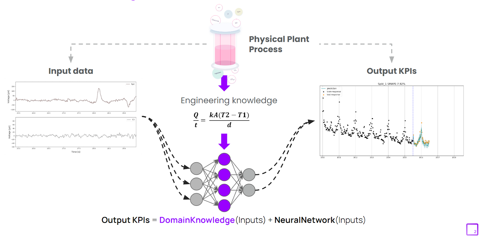
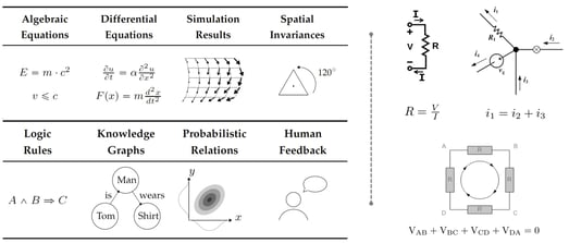
In other words, physics establishes our known system dynamics,  while ML fills in the gaps of our established physics models/knowledge. Physics-based models can be as simple as mass balance rules (i.e., the sum of inputs is equal to the sum of outputs), or a full set of partial differential equations that describe the evolution of a system (i.e. protein binding on chromatography column).

How to Embed Domain Knowledge into Machine Learning

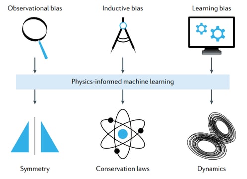
There are 3 general ways to embed domain knowledge with ML which will be described in subsequent sections [1]:

1. Introducing observational bias to the data
2. Introducing inductive bias into the model structure
3. Introducing learning bias to how models are trained

‍

‍

‍

‍

‍

1. Introducing Observational Bias

Observational biases can be introduced directly through data that embody the underlying physics or via data cleaning and processing. Essentially, a data scientist or engineer filters the process data for the subset(s) that represents the particle physical system the best.
This represents the simplest mode of introducing biases in ML when dealing with large volumes of data. This process is typically necessary to generate predictions that respect certain symmetries and dynamics of the underlying process.
This method can be quite challenging for industrial digital twin applications, since it requires significant data preprocessing and manipulation that isn’t always feasible in industrial environments.

2. Introducing Inductive Bias

Inductive biases correspond to prior assumptions that can be incorporated by tailored interventions to an ML model architecture, such that the predictions sought are guaranteed to implicitly satisfy a set of given physical laws, typically expressed in the form of certain mathematical constraints. Essentially, one can change the architecture of the ML model to match the expectation of the underlying physics of the process.

Despite their high effectiveness, such approaches are currently limited to tasks that are characterized by relatively simple and well-defined physics or symmetry groups , and often require significant subject matter expertise and elaborate implementations [1].

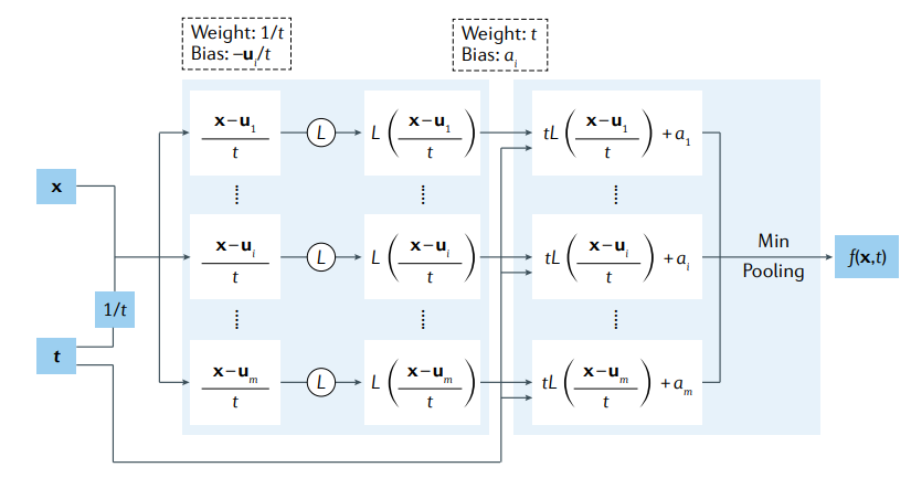
Moreover, their extension to more complex tasks is challenging, as the underlying invariances that characterize many physical systems are often poorly understood or hard to implicitly encode in a neural architecture. Specifically for solving differential equations using neural networks, architectures can be modified to satisfy exactly the required initial conditions [1]. In addition, if  some features of the PDE solutions are known a priori, it is  also possible to encode them in network architectures [1].

3. Introducing Learning Bias

Instead of designing a specialized architecture that implicitly enforces domain knowledge, modern implementations aim to impose such constraints in a soft manner by appropriately penalizing the loss function of conventional neural networks [1].

This approach can be viewed as a specific use-case of multi-task learning, in which a learning algorithm is simultaneously constrained to fit the observed data, and to yield predictions that approximately satisfy a given set of physical constraints. This provides a very flexible platform for introducing a broad class of domain-driven biases that can be expressed in the form of algebraic or differential equations.

Representative examples of learning bias approaches include physics-informed neural networks (PINNs) and their variants.

Physics Informed Neural Networks (PINNs)

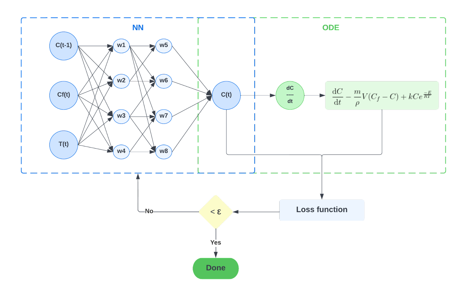
Physics-informed neural networks (PINNs) integrate information from both real-world measurements and mechanistic models - i.e. ordinary or partial differential equations (ODEs/PDEs). This integration is achieved by embedding the ODEs/PDEs into the loss function of a neural network using automatic differentiation.

We present the PINN algorithm for solving forward problems using the example of a completely stirred reactor (CSTR) for chemical production.

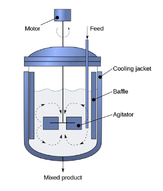
Here, we assume that the motorized agitator within the CSTR will create an environment of perfect mixing within the vessel. We further assume that the product stream will have the same concentration and temperature as the reactor fluid. To keep the reaction chemistry relatively simple, we assume first order reaction kinetics. We also excluded the energy balance in this analysis.

A simple mass balance of the product concentration stream yields the following ordinary differential equation (ODE):

The summary of terms used in the above ODE are listed in the table below.

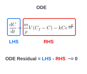
By subtracting the right hand side of the ODE from its left hand side, we can compute the residual or loss term for the ODE. In a typical mechanistic model fitting application, one would aim to calibrate this model by fitting various model parameters to actual plant measurements. This involves substituting true measurements of C_f, C and T retrieved from historical data and computing the derivative of C in order to minimize the residual/loss of the ODE.

To embed the ODE into a neural network’s framework, we append the supervised loss of data measurements of C with the aforementioned unsupervised loss of the ODE:

‍

‍

‍

‍

w_data and w_ODE  are the weights used to balance the interplay between the two loss terms. These weights can be user-defined or tuned automatically, and play an important role in improving the trainability of PINNs [1,7]. The network is trained by minimizing the loss via gradient-based optimizers, such as Adam and L-BFGS, until the loss is smaller than a user defined threshold ε.

‍

Conclusion

Physics-informed Machine Learning (PIML) is the process of embedding established domain knowledge with ML to accurately model dynamic industrial systems. There are 3 general ways to embed domain knowledge with ML, including:

• Introducing observational bias to the data
• Introducing inductive bias into the model structure
• Introducing learning bias to how models are trained

Physics-informed neural networks (PINNs) are a novel approach that integrate the information from both process data and engineering knowledge by embedding the ODEs into the loss function of a neural network. PIML integrates data and mathematical models seamlessly even in noisy and high- dimensional contexts.Thanks to its natural capability of blending physical models and data as well as the use of automatic differentiation, PIML is well placed to become an enabling catalyst in the emerging era of digital twins. [1]

If you're interested in learning more about hybrid modelling and how companies like Basetwo are helping manufacturers rapidly adopt and scale modelling technologies, feel free to check out our use cases and white papers on our resource page.

References:

- Karniadakis, G.E., Kevrekidis, I.G., Lu, L. et al. Physics-informed machine learning. Nature Rev Phys 3, 422–440 (2021).
- L. von Rueden et al. Informed Machine Learning — A Taxonomy and Survey of Integrating Prior Knowledge into Learning Systems. IEEE Transactions on Knowledge and Data Engineering (2021)
- Lu, L., Jin, P., Pang, G., Zhang, Z. & Karniadakis, G. E. Learning nonlinear operators via DeepONet based on the universal approximation theorem of operators. Nat. Mach. Intell. 3, 218–229 (2021)
- Li, Z. et al. Fourier neural operator for parametric partial differential equations. in Int. Conf. Learn. Represent. (2021).
- Yang, Y. & Perdikaris, P. Conditional deep surrogate models for stochastic, high-dimensional, and multi-fidelity systems. Comput. Mech. 64, 417–434 (2019)
- Lagaris, I. E., Likas, A. & Fotiadis, D. I. Artificial neural networks for solving ordinary and partial differential equations. IEEE Trans. Neural Netw. 9, 987–1000 (1998)
- Mattheakis, M., Protopapas, P., Sondak, D., Di Giovanni, M. & Kaxiras, E. Physical symmetries embedded in neural networks. Preprint at arXiv: https://arxiv.org/abs/1904.08991 (2019)
- Zhang, D., Guo, L. & Karniadakis, G. E. Learning in modal space: solving time-dependent stochastic PDEs using physics-informed neural networks. SIAM J. Sci. Comput. 42, A639–A665 (2020)
- Darbon, J. & Meng, T. On some neural network architectures that can represent viscosity solutions of certain high dimensional Hamilton-Jacobi partial differential equations. J. Comput. Phys. 425, 109907 (2021).
- Raissi, M., Perdikaris, P. & Karniadakis, G. E. Physics-informed neural networks: a deep learning framework for solving forward and inverse problems involving nonlinear partial differential equations. J. Comput. Phys. 378, 686–707 (2019).
- Lagaris, I. E., Likas, A. & Fotiadis, D. I. Artificial neural networks for solving ordinary and partial differential equations. IEEE Trans. Neural Netw. 9, 987–1000 (1998).
- Zhang, D., Guo, L. & Karniadakis, G. E. Learning in modal space: solving time-dependent stochastic PDEs using physics-informed neural networks. SIAM J. Sci. Comput. 42, A639–A665 (2020).
- Kissas, G. et al. Machine learning in cardiovascular flows modeling: predicting arterial blood pressure from non-invasive 4D flow MRI data using physics informed neural networks. Comput. Methods Appl. Mech. Eng. 358, 112623 (2020).
- Zhu, Y., Zabaras, N., Koutsourelakis, P. S. & Perdikaris, P. Physics-constrained deep learning for high-dimensional surrogate modeling and uncertainty quantification without labeled data. J. Comput. Phys. 394, 56–81 (2019).
- Geneva, N. & Zabaras, N. Modeling the dynamics of PDE systems with physics-constrained deep auto-regressive networks. J. Comput. Phys. 403, 109056 (2020).
- Wu, J. L. et al. Enforcing statistical constraints in generative adversarial networks for modeling chaotic dynamical systems. J. Comput. Phys. 406, 109209 (2020).
- Wang, S., Yu, X. & Perdikaris, P. When and why PINNs fail to train: a neural tangent kernel perspective. Preprint at arXiv https://arxiv.org/abs/2007.14527 (2020).
- Yang, L., Zhang, D. & Karniadakis, G. E. Physics-informed generative adversarial networks for stochastic differential equations. SIAM J. Sci. Comput. 42, A292–A317 (2020).
- Pang, G., Lu, L. & Karniadakis, G. E. fPINNs: fractional physics-informed neural networks. SIAM J. Sci. Comput. 41, A2603–A2626 (2019).
- Lu, L., Meng, X., Mao, Z. & Karniadakis, G. E. DeepXDE: a deep learning library for solving differential equations. SIAM Rev. 63, 208–228 (2021).
- Wang, S., Teng, Y. & Perdikaris, P. Understanding and mitigating gradient pathologies in physics-informed neural networks. Preprint at arXiv https://arxiv.org/ abs/2001.04536 (2020).